Low Rank Adaptations. What are they, implementation and are they useful in smaller models?
Low Rank Adaptations (LoRA) are a hot topic in deep learning, specially for huge models like GPT-3 or StableDiffusion. In summary, LoRA allows for efficient adaptation of large language models by introducing trainable rank decomposition matrices while keeping the pretrained weights frozen. It reduces the number of trainable parameters, memory requirements, and hardware barriers while maintaining or improving model quality compared to full fine-tuning. It’s a simple method that I think it’s smart and very interesting for democratizing AI.
However, existing implementations like https://github.com/huggingface/peft use this technique with models like RoBERTa in their examples, and in my experience this has little impact. I decided to check whether this makes any difference in terms of throughtput performance (not checking metrics like accuracy) for these models’ scales. Keep in mind that this post is a rough estimate, since I don’t have access to large computing.
What are Low Rank Adaptations?
LoRA is one of the so called ‘side-tuning’/‘fine-tuning’. The benefit it brings into the table is that it has no lattency during inference, as opposed to some techniques as Adapters, and allows to tune the whole matrix as opposed to some other methods like bitfit.
The method comes from the idea that LLMs are overparametrized, so the set of parameters for any layer can be expressed by a combination of a lower rank parameter space. Take for example an attention matrix, in particular the weight matrix for the query $W_q$ of dimensions $e \times h$ (embedding dimension times hidden dimension).
Instead of fine-tuning the $W_q$ matrix itself, LoRA proposes to freeze that matrix and fine tune two new matrices of dimensions $e \times r$ and $r \times h$, with $r$ being a low rank value (i.e. 3)
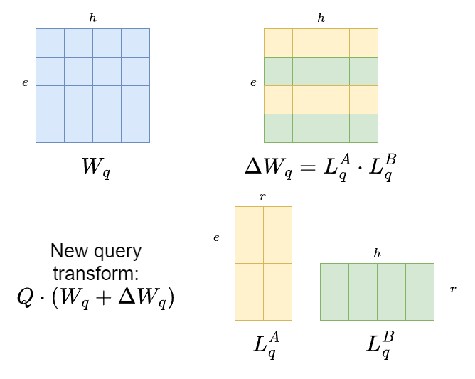
Then, when doing inference, the calculations times are the same because you will only have in memory the addition of the two matrices, which will be the same as fine tuning!
Another interesting point is savings in memory. You can have your big model with $W_q$ and then have one $\delta W_q^t$ for each one of your tasks, so each task is represented by a separate, addable, lightweight matrix.
You also have to compute way less gradients (for an $e=100, h=100, r=2$ matrix with $e \times h = 10000$ original parameters you would be tuning just $er + rh=200$ parameters).
However, not everything is rosy. For small models (thanks to Pedro Cuenca and Younes Belkada, authors of the great blogpost explaining the method https://huggingface.co/blog/lora that pointed me towards this) the computational overhead of the $L$ matrices multiplication might not compensate the fact that you are computing less gradients.
Let’s check this with a practical example. I’ll be using Distilbert and RoBERTa-scale parameters, since it’s as much as I can afford with the gpu I have at home.
Setting up our benchmark
Some imports to make our life easier plus a little decorator that will help us time functions
import matplotlib.pyplot as plt

from itertools import product
from functools import wraps
from random import choices, seed
from time import time
from numpy import median, nan
from loguru import logger
import pandas as pd
from tqdm import tqdm
seed(123456)
skip_loop = True

def with_timing(return_t: bool = False, log: bool = True):
    """Decorator that times a function.

    It allows the user to retrieve or log the timing

    Args:
        return_t (bool, optional): If true, returns a (time, result) tuple
        log (bool, optional): If true, logs the time through loguru's logger
    """
    def decorator(f):
        @wraps(f)
        def wrap(*args, **kwargs):
            t0 = time()
            result = f(*args, **kwargs)
            tdiff = time() - t0
            if log:
                logger.info(f"{f.__name__} took {tdiff:.5f}s")
            return (result, tdiff) if return_t else result

        return wrap

    return decorator
Implementing the attention mechanism
from jax import jit, grad, vmap, numpy as jnp, random, nn

def random_setup(
    batch_size: int,
    embedding_dim: int,
    hidden_dim: int
):
    """Returns X and Wk, Wq, Wv matrices"""
    key = random.PRNGKey(0)
    keys = random.split(key,4)

    X = random.uniform(keys[0], (batch_size, embedding_dim))
    setup = [X]
    for key in keys[1:]:
        att_shape = (embedding_dim, hidden_dim)
        setup.append(random.uniform(key, att_shape))

    return setup

def random_lora_setup(
    embedding_dim: int,
    hidden_dim: int,
    r: int
):
    """Returns l_WkA, l_WkB,l_WqA, l_WqB LoRA matrices"""
    key = random.PRNGKey(0)
    keys = random.split(key,2)

    setup = []
    for key in keys:
        l_A = random.uniform(key, (embedding_dim, r))
        l_B = random.uniform(key, (r, hidden_dim))
        setup.extend([l_A, l_B])

    return setup

@jit
def self_attention(
    X: jnp.ndarray,
    Wk: jnp.ndarray,
    Wq: jnp.ndarray,
    Wv: jnp.ndarray
):
    X = jnp.atleast_2d(X)
    Q = X @ Wq
    K = X @ Wk
    V = X @ Wv
    dk = Wv.shape[-1]
    att_weights = jnp.dot(Q, K.T) / dk**.5
    att_weights = nn.softmax(att_weights)
    return jnp.dot(att_weights,V)

@jit
def lora_self_attention(
    X: jnp.ndarray,
    Wk: jnp.ndarray,
    Wq: jnp.ndarray,
    Wv: jnp.ndarray,
    l_WkA: jnp.ndarray,
    l_WkB: jnp.ndarray,
    l_WqA: jnp.ndarray,
    l_WqB: jnp.ndarray,
):
    delta_Wk = l_WkA @ l_WkB
    delta_Wq = l_WqA @ l_WkB

    return self_attention(
        X,
        Wk + delta_Wk,
        Wq + delta_Wq,
        Wv
    )

def loss_f(f, *args, **kwargs):
    @jit
    def loss(*args, **kwargs):
        return f(*args, **kwargs).sum()
    return loss

@with_timing(return_t=True, log=False)
def test_vanilla(X, Wk, Wq, Wv):
    forward = self_attention(X, Wk, Wq, Wv)
    loss = loss_f(self_attention)
    backward = grad(loss, [1,2,3])(X, Wk, Wq, Wv)


@with_timing(return_t=True, log=False)
def test_lora(X, Wk, Wq, Wv, l_WkA, l_WkB,l_WqA, l_WqB):
    forward = lora_self_attention(X, Wk, Wq, Wv, l_WkA, l_WkB,l_WqA, l_WqB)
    loss = loss_f(lora_self_attention)
    backward = grad(loss, [4,5,6,7])(X, Wk, Wq, Wv, l_WkA, l_WkB,l_WqA, l_WqB)
In each test, I’ll run a forward-backward pass of the method. I’ve been explicitly verbose with the parameters in order to make code easily readable
batch_sizes = [2, 64, 256, 1024]
embedding_dims = [256, 512, 1024, 2048]
hidden_dims = [256, 512, 1024, 2048]
low_ranks = [1,3,5]

setups = list(product(batch_sizes, embedding_dims, hidden_dims, low_ranks))
if skip_loop:
    setups = []
results = {'vanilla':{}, 'lora':{}}
for i, setup in enumerate(tqdm(setups)):

    batch_size, embedding_dim, hidden_dim, low_rank = setup
    vanilla_params = random_setup(batch_size, embedding_dim, hidden_dim)
    lora_params = random_lora_setup(embedding_dim, hidden_dim, r=low_rank)

    t_v = 0
    t_l = 0
    for _ in range(10):
      _, t_vi = test_vanilla(*vanilla_params)
      _, t_li = test_lora(*vanilla_params, *lora_params)

      t_v += t_vi/10
      t_l += t_li/10

    results['vanilla'][setup] = t_v
    results['lora'][setup] = t_l


    pd.DataFrame(results).to_csv('results.csv')
Here I’m loading some results I obtained with a GPU
df = pd.read_csv('results_gpu.csv')
factors = ["batch_size", "embedding_dim", "hidden_dim", "low_rank"]
outcomes = ["vanilla", "lora"]
df.columns = factors + outcomes
df[factors] = df[factors].astype(int)
df['diff'] = df['lora'] - df['vanilla']
from itertools import product, combinations
paste = '_'.join
f_combinations = map(list, combinations(factors, 2))
for f_comb in f_combinations:
    for outcome in outcomes:
        mean = df.groupby(f_comb)[outcome].median().reset_index()
        x = mean[f_comb].astype('str').apply(paste, axis=1)
        plt.bar(x, mean[outcome], label=outcome, alpha=0.5)
        plt.xticks(x, rotation='vertical')
        plt.xlabel(paste(f_comb))
    plt.legend()
    plt.show()
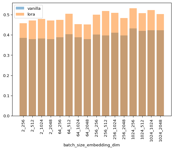
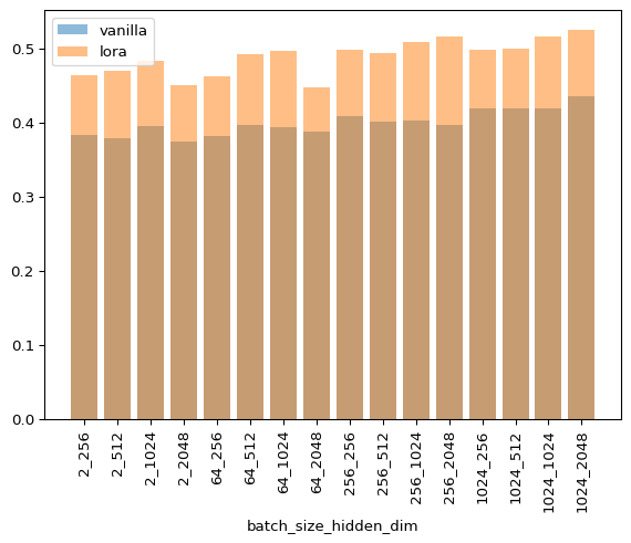
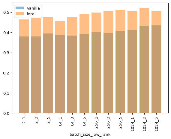
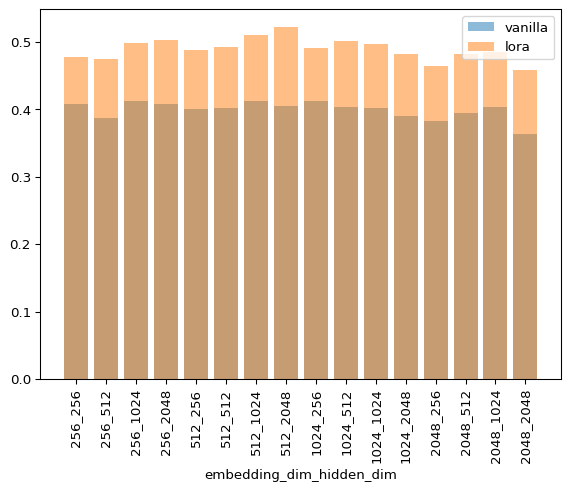
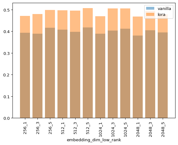
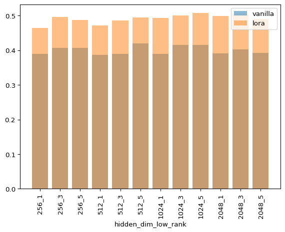
As you can see, LoRA is never faster for any combination of hyperparameters. I’m not discarding that my implementation can be more efficient as I’m still a JAX novice, but this matches my empirical experience when fine tuning models of this size.
As you know, GPT models have hidden sizes of up to 50k, and I can’t play in that and run experiments in that league with an 8 year old GPU and collab. But the authors of LoRA report approx. a 40tokens/s vs 30tokens/s increase, so that’s a big number for a simple method!
Thanks for reading and if you want to comment something I’m happy to listen!
